[STRAUS Applications] [STRAUS Specifications]
[STRAUS Users Page] [STRAUS Model Archive] [Technical Papers and Tips Contents Page]
[Technical Articles Contents Page] [Home Page] [Previous Page] [Next Page]

Modelling Structures with Rigid Body Motion

For the majority of Linear Static runs, we can find some part of the structure which can be rigidly fixed in space in order to prevent rigid body motion. When such a point cannot be easily identified, a different approach can be taken that allows us to solve a free floating structure, provided the applied forces are in equilibrium. For this we use the Transient Dynamic Solver. This solver adds a new dimension to the analysis; that of time. If we are solving in the time domain our structure does not need to be fixed in space. Consider the following simple problem:

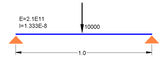
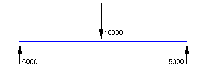
A simply supported beam has a tip load applied to the centre as shown above. Usually we would solve this using the linear static solver by applying appropriate freedom conditions at the ends. To use the Transient Solver we need to determine the reactions and apply these instead of restraints. The model will then look like the following figure.

To solve this with the transient solver we need to define a number of new parameters in the solver options panel. These include the Time Step, the Damping Coeeficient and the Load Vs time Tables.

Since we are not really interested in the dynamic behaviour of the structure, the time step is not critical. Although we can determine a "correct" time step by looking at the period of the first natural frequency, we can usually guess a time step by having a rough idea of the frequencies in the structure. For the model above, a time step of 0.01 seconds was used. We need also to enter the total number of time steps for the transient. In this example, 10 steps were used giving us a total solution time of 0.1 seconds.

Next we need to aply some damping to the system. Without damping, the structure will never come to rest and will simply settle down to some oscillatory behaviour. For this model we use Rayleigh Damping with factors of 1.0. These factors should be applied at frequencies close to the first natural frequency such that the structure comes to rest as soon as possible. Note that to include Rayleigh damping, you should enter a density for the material.

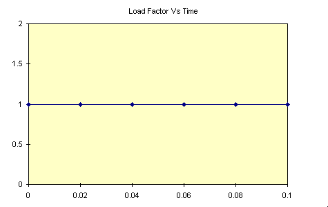
Now we need to describe the behaviour of the load vs time. The load is instantaneoulsly applied at time zero and kept constant for all time. A Load Vs Time Table as shown below was used. Note that the time span of the table must be sufficiently large to cover the total time span for which the solver is run; ie. the time step multiplied by the number of steps used.

The results of this run are illustrated in the following graph.

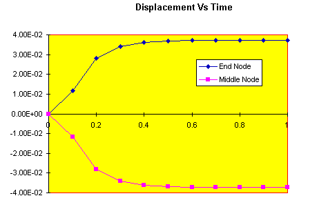
This shows the displacement of the mid span of the beam, and at one end of the beam, for each time step. The total deformational displacement is given by the difference between the two lines. We see that at infinte time (or 0.1s in this case) a total deformation of 74.38 is obtained. Engineer's theory of Bending gives 74.4 for this beam (which is the same value given by the linear Static Solver).

For more information please contact us by e-mail: hsh@iperv.it