[STRAUS Applications] [STRAUS Specifications]
[STRAUS Users Page] [STRAUS Model Archive] [Home Page] [Technical Papers and Tips Contents Pages]

Conservative and Non-Conservative Loads
Zero Stresses on Plate Models
Plate Element Orientation
Local Vs Global Stesses in Plates
Ambient Vs Reference Temperature
Direct Summation of Loads
Non Linear Analysis - Setting Up the Load Table

Conservative and Non-Conservative Loads

STRAUS has provisions for both of these. Point loads and moments and global accelerations are conservative as these are independent of the structure on which they act. They always act in directions given by the global coordinate system. Element attributes such as UDLs (uniformly distributed loads) on beams, plate and brick pressures etc., are non-conservative. These always act relative to the element's local coordinate system and in geometric nonlinear analysis, the loads follow the elements.

Zero Stresses on Plate Models

Sometimes a contour plot of stresses on a plate mode shows zero stress, even though the plate has deflected. This is usually because you are looking at the stresses on the plate's mid plane. If the problem is a pure bending problem, ie. there is no membrane action, then the stresses will be zero at the neutral plane of the plate. The neutral plane is the default STRAUS location for contouring and peeking at stresses. With this thpe of problem you should be looking at the stresses on the upper and lower surfaces of the plate (ie. the +z and -z locations).

Plate Element Orientation

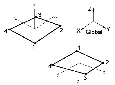
When looking at plate surface stresses, it is important that the elements be orientated correctly with respect to each other. Associated with each element is a local coordinate system, denoted by x-y-z in STRAUS. The x and y axes lie in the plane of the plate and the z axis is normal to the plate's surface as shown below. It is important that the local z axis point in the same direction for adjoining plates otherwise contour plots of suface stress can be meaningless. To check your plate's orientation, simply set the plate display type to ORIENTATION and redraw.

Local Vs Global Stresses in Plates

Whenever you produce a contour plot of stresses or peek at nodestresses, you have the option of local stresses (denoted by lower case subscripts) or global stressees (denoted by upper case subscripts). The lower case values refer to stresses in the local element system shown above. This depends on the numbering order on the element and is usually different from element to element. The upper case values refer to the stresses in the global X-Y-Z system and this direction is invariant from element to element.

In a flat plate structure, where the elements lie on one of the global coordinate planes (eg. XY or YZ or ZX planes), it is usually more informative to look at the globally directed stresses. This is appropriate for a concrete slab (say). There are cases where the local stresses are very useful, such as in the following figure, provided care had been taken to properly orientate the elements.

As shown in the figure, the elements have been numbered in such a way that the local y axis follows the contour of the mesh. Here a plot of local y stresses will give the stresses in a direction indicated by the mid line in the mesh above.

Note that for a general 3D shell structure, neither of the two methods is useful. The global stresses cannot be used because the shell will not lie on a global plane. Contours of the local stresses are also of little use since it is unlikely that the elements could be correctly orientated. In such cases principal stress contours and principal stress vectors (which also show the direction of maximum stress) are more informative. If detailed stresses are required, then individual elements should be investigated separately.

Ambient Vs Reference Temperature

Structural Solver
The Structural Solver uses the Reference Temperature (in the Global Data Panel) to calculate the change in temperature at each node such that a strain equal to alpha time temperature change is applied (alpha is the termal expansion coefficient). The change in temperature is given by the temperature assigned to the node minus the Reference Temperature. The structural Solver does not make use of the Ambient Temperature (defined in the element's property screens).

Heat Solver
The Heat solver uses the Reference Temperature only in Transient problems. For Steady State Heat Flow, the Reference Temperature is not used. In a Transient Heat Problem, the Reference Temperature is used as the inital temperature of all nodes which are not set to some other temperature. The Ambient Temperature is used by all the Heat Solvers. This is the temperature of the surroundings. With this arrangement, it is very easy to analyse a structure which starts at elevated temperature (the Reference Temperature) and then allowed to progressively cool to the Ambient Temperature.

Direct Summation of Loads

When you execute the linear or nonlinear static solvers, STRAUS reports the total amount of load acting on the structure as:

1. DIRECT SUMMATION
2. MOMENTS ABOUT THE ORIGIN

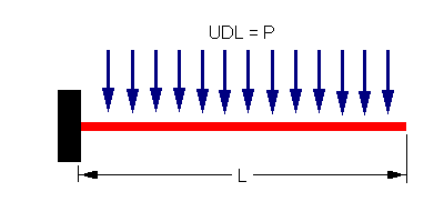
These numbers can be very useful in monitoring the amount of load you have actually applied to the structure, and for checking overall equilibrium with recoverd reactions. The MOMENTS ABOUT THE ORIGIN reports the total moment sum (MX,MY,MZ) about a point at (0,0,0). The direct summation on the other hand, is often misinterpreted; it is simply the summation of the entries in the RHS vector {P} in the equation [K]{d}={P}. This means that on a structure where there is a zero net force, (e.g. a cylinder with a uniform internal pressure), the (FX,FY,FZ) values will be reported as zero. In addition, the moments (MX,MY,MZ) listed here will be different from those given by the MOMENTS ABOUT THE ORIGIN because they do not include the moments due to forces. Further, because the values listed are the summation of the loads in {P}, this does not include any load which is applied to contrained nodes. This means that on the structure shown in the following picture, the total FY is reported as 0.5PL instead of the expected PL.

Cantilever with uniform distributed load.

Non Linear Analysis - Setting Up the Load Table

For those who are just starting out in nonlinear analysis it is important that you understand the function of the load tables.

In nonlinear analysis the loads are applied incrementally, that is the load is stepped up gradually and convergence achieved at each level of load before applying further load. This is necessary to ensure stability and convergence of the solution.

Many new users of the nonlinear solver are unsure of the requirements for setting up this load table. There are basically three things that must be considered - the number of increments, the number of iterations and the proportion of the load that is applied in each increment.

For material nonlinear analysis the entire load is normally applied in one load increment and many iterations are used to ensure convergence. For geometric nonlinear analysis the requirements are different.

The default number of increments in the solver panel is 10. Users can however select any number of increments within the range of 1-100. The number of increments required is dependent on the degree of nonlinearity in the structure.

For a typical civil/structural engineering problem where nonlinear P-D effects are to be considered the load table will typically only have about 3-4 increments. Such problems only involve small nonlinearities since the deflections are still essentially small. This means that the load can be applied relatively quickly. The main effect being considered in such problems is the redistribution of load that occurs as a result of the small deflections. On the other hand structures that involve complex nonlinearities such as buckling or structures with large deflections, (eg. membranes), can require many increments.

The exact number of increments required for a particular problem is difficult to estimate and must really be determined by the experience of the user and/or trial and error.

The number of iterations required must be sufficient to ensure convergence for a given load increment. The number of iterations specified by the user only defines the maximum number at which the solution is terminated for a particular load increment. Of course if the solution converges in less than the number specified then only those iterations actually required are carried out.

The most difficult part of the load table to get right is the magnitude of the load factors. In many cases it is sufficient to divide the load equally between the different load increments. However this may not provide optimum convergence and in some cases may not allow the solution to converge at all. If you do not have a feeling for the required magnitude of the load increments then you probably should start with equal load increments.

There are many types of nonlinear analysis where a constant load step is undesirable nor optimum. An example is a problem that involves nonlinear buckling. The model can initially be loaded quite rapidly until the load level is just below the buckling load. As the buckling load is approached the size of the load steps is reduced until very small steps are used to capture the formation of the buckle.

Another case where nonuniform stepping is essential is in the solution of some cable and membrane problems. This type of problem requires a table which is the opposite of that required for the buckling problem. The cable or membrane initially has no stiffness and the load is initially applied in small steps to allow the deflection and hence stiffness of the structure to develop gradually. Once the structure has assumed the basic deformed shape the loads can be applied more rapidly.

It can be seen from the above that setting up the load table requires a knowledge of the function of the table and also of the likely behaviour of the structure. It is obviously a task that will become easier when the user has had some experience. To a certain extent the load table requires a degree of experimentation on the part of the user. Even experienced users will find it necessary to experiment a little to achieve optimum convergence for a particular problem.

In the next release of STRAUS, we have included an automatic step halving capability, such that the solver will reduce the amount of load applied if convergence cannot be achieved.

For more information please contact us by e-mail: hsh@iperv.it